snakeplot

Sequential data tells a story—survey items build on each other, career phases unfold over time, learning activities chain into patterns. Conventional plots break these sequences into disconnected bars or points, losing the thread that connects them. A long sequence plotted as a single horizontal strip forces the reader to scroll or squint at a compressed axis; a vertical list wastes space and hides adjacency. snakeplot solves this by winding data through a serpentine layout where each row flows into the next through U-turn arcs, keeping the full sequence visible, connected, and compact in a single figure—much like reading lines of text on a page.

Timeline: A career in one glance

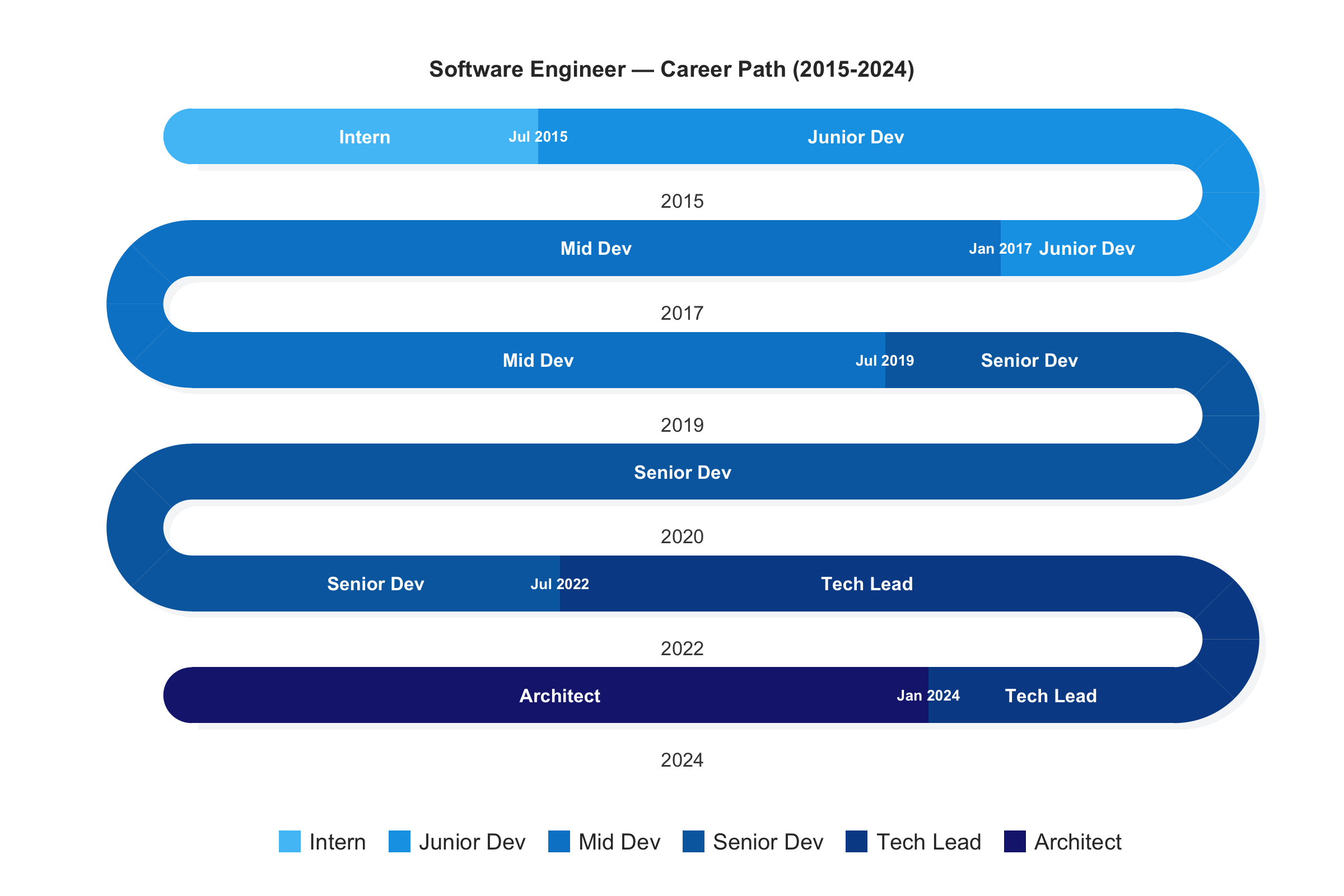
A 10-year career plotted as a conventional horizontal timeline either stretches too wide to fit on a page or compresses short phases into unreadable slivers. The serpentine layout folds the timeline into stacked bands—each band covers roughly two years, and the eye simply reads left-to-right, then right-to-left on the next row, like text. Transitions are labeled at the exact month they occur, year markers sit below each band, and a sequential palette darkens with seniority—so the entire career arc is visible in one compact figure. timeline_snake() takes a simple 3-column data.frame (role, start, end) and handles all the date arithmetic automatically.

career <- data.frame(
  role  = c("Intern", "Junior Dev", "Mid Dev",
            "Senior Dev", "Tech Lead", "Architect"),
  start = c("2015-01", "2015-07", "2017-01",
            "2019-07", "2022-07", "2024-01"),
  end   = c("2015-06", "2016-12", "2019-06",
            "2022-06", "2023-12", "2024-12")
)
timeline_snake(career,
               title = "Software Engineer — Career Path (2015-2024)")

State sequences: 75 events as a continuous path

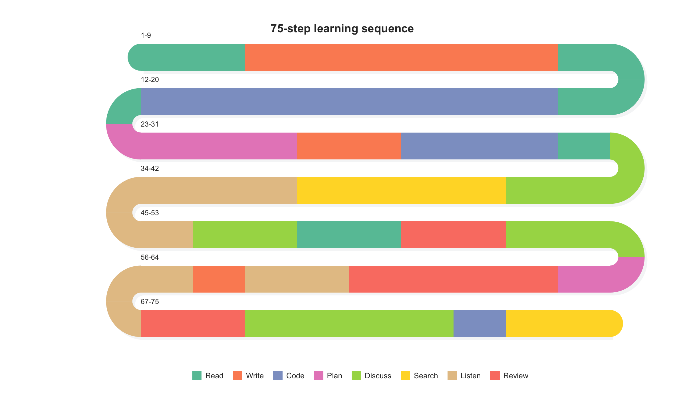
A 75-step sequence plotted as a single row of colored blocks would stretch far beyond screen width, forcing scrolling and making it impossible to see the overall pattern. Stacking the same data as vertical bars loses the left-to-right reading order that makes sequences intuitive. The serpentine layout solves both problems: it folds the sequence into readable bands connected by U-turn arcs, so the full path stays visible in one figure. Runs of the same state are visually immediate as colored stretches; transitions pop out as color boundaries. No information is lost, no order is scrambled—the reader traces the path exactly as the events unfolded.

sequence_snake(seq75, title = "75-step learning sequence")

Surveys: Inter-item correlations at U-turns

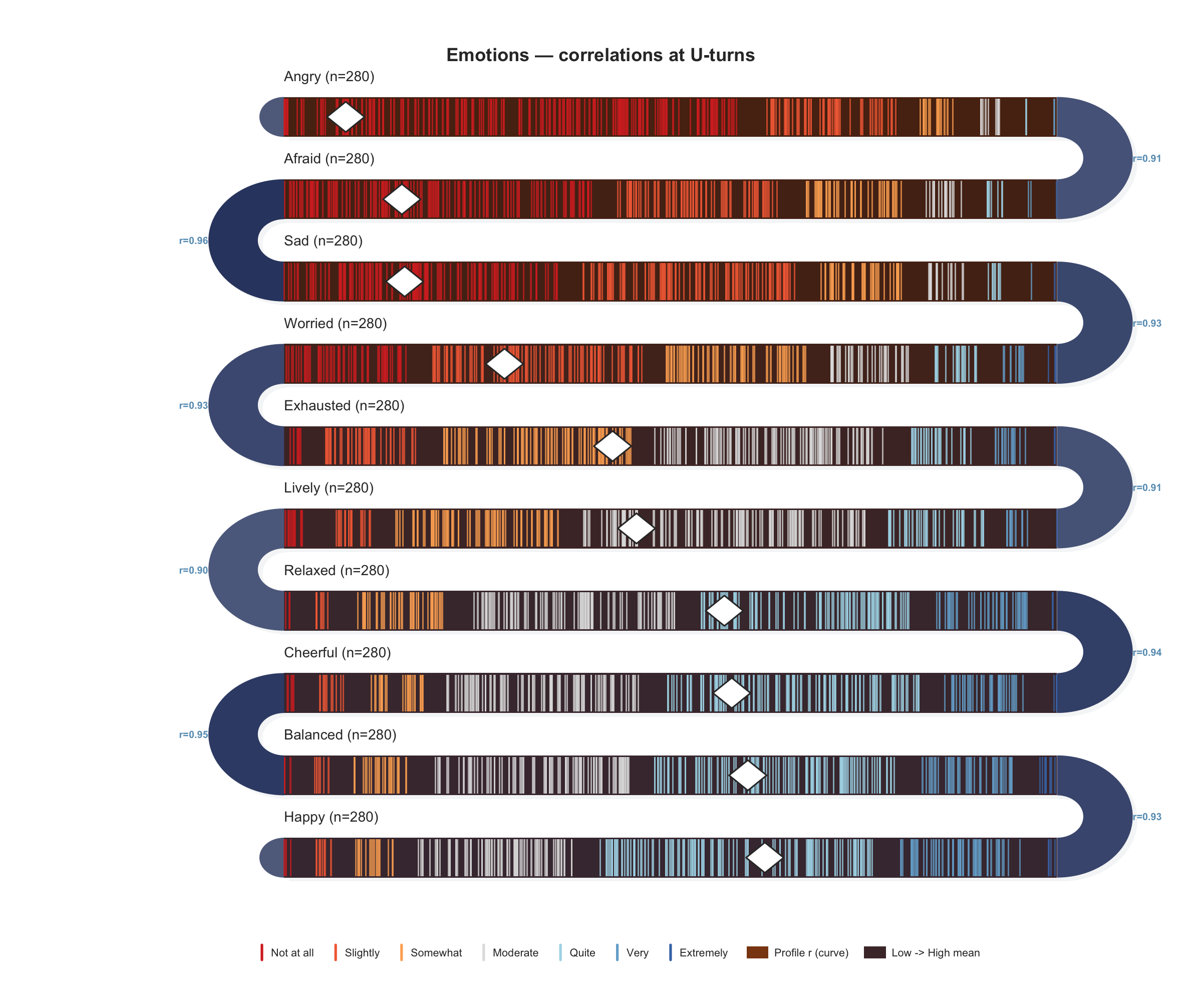
A survey with 15+ items sorted by mean creates a natural ranking, but standard bar charts show only summary statistics and strip charts show only raw responses—neither reveals how adjacent items relate to each other. The serpentine layout turns that adjacency into an asset: the U-turn arc connecting two neighboring items becomes a space to display their Pearson correlation, so you see both the item-level distributions and the inter-item structure in one figure. Brown arcs signal positive association, blue arcs signal negative—anomalous pairs stand out immediately without consulting a separate correlation matrix.

survey_snake(ema_emotions, tick_shape = "line",
             arc_fill = "correlation", sort_by = "mean",
             colors = snake_palettes$ocean, level_labels = labs7,
             title = "Emotions — correlations at U-turns")

Response distributions as stacked bars

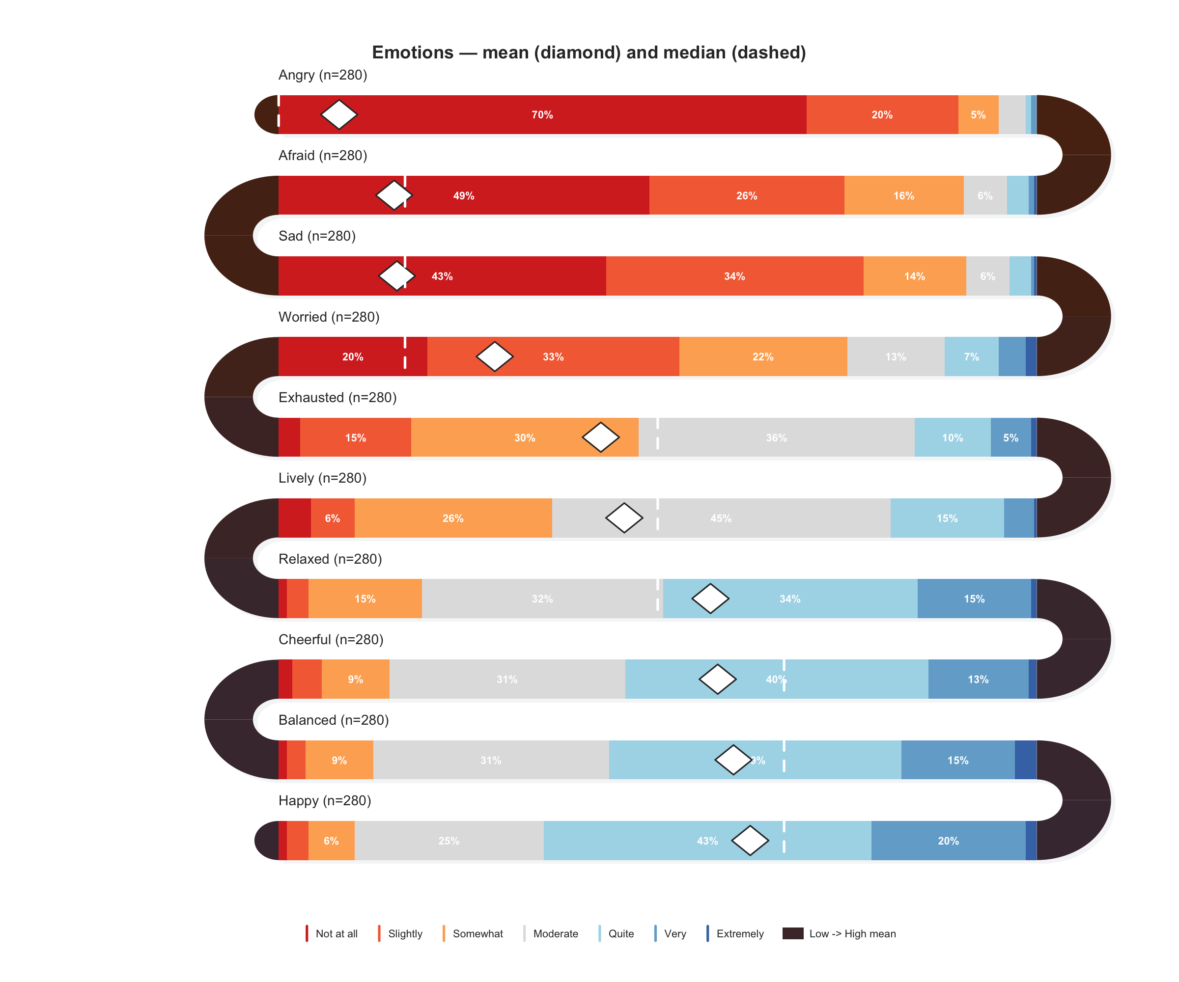
When the question shifts from “how do individual responses scatter?” to “what is the overall distribution shape?”, switching to tick_shape = "bar" renders each item as a 100% stacked bar. Sorting by mean turns the serpentine into a gradient—from the most negatively rated item to the most positive—so you can spot where the distribution shifts from skewed-low to skewed-high. Mean diamonds and median lines overlay summary statistics directly on the bars, replacing the need for a separate descriptive table.

survey_snake(ema_emotions, tick_shape = "bar", sort_by = "mean",
             show_mean = TRUE, show_median = TRUE,
             colors = snake_palettes$ocean, level_labels = labs7,
             title = "Emotions — mean and median markers")

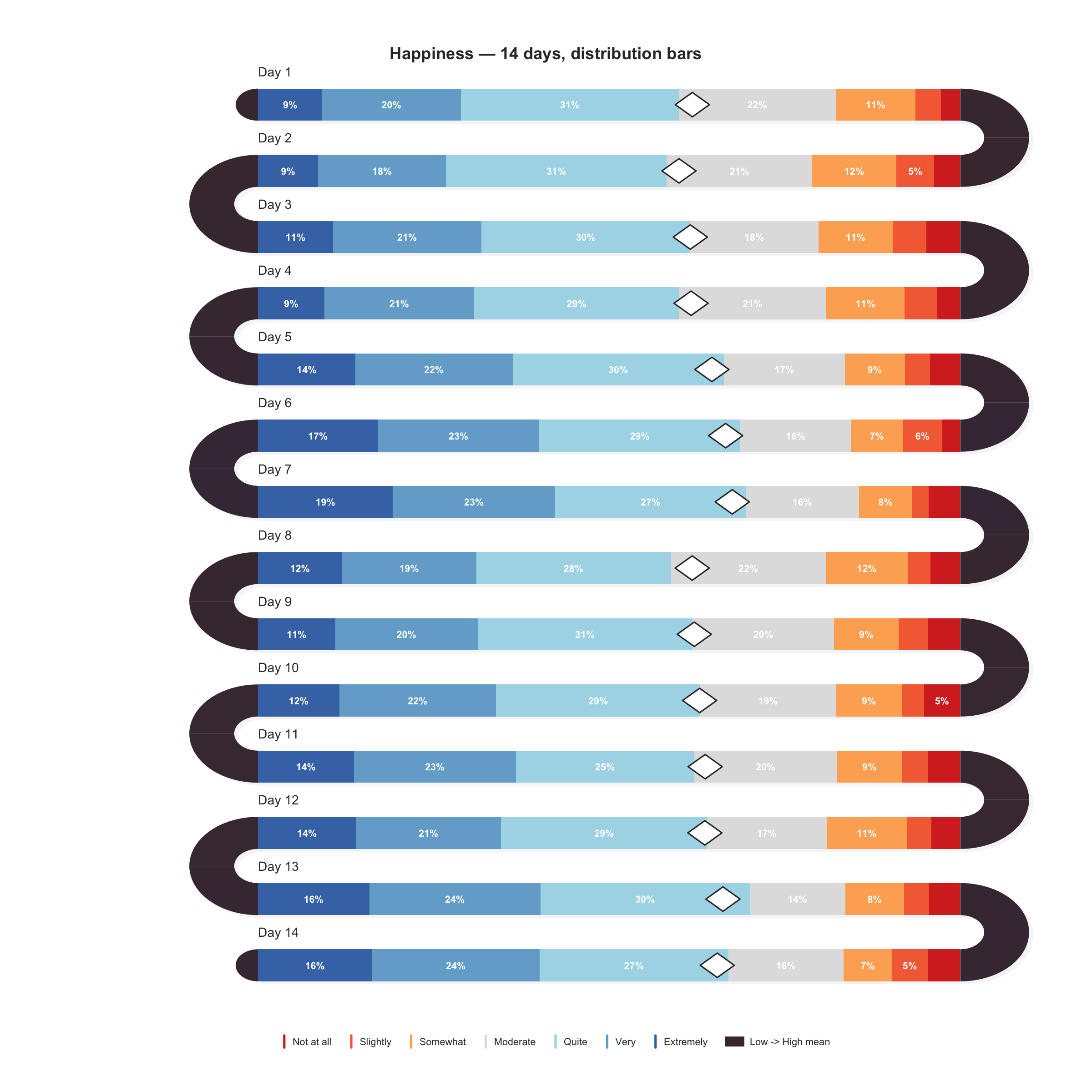
Daily EMA: 14 days of experience sampling

Experience sampling studies generate beep-level data across many days—14 days of 5–10 beeps each produces 70–140 observations that need to be compared both within and across days. Faceted panels lose the day-to-day continuity; a single long axis compresses each day into a narrow slice. The serpentine layout gives each day its own full-width band, and the U-turn arcs connect consecutive days so you can trace how distributions shift from Monday to Sunday. Within-day patterns (morning dips, evening peaks) are visible within each band, while between-day trends emerge across bands.

survey_snake(ema_beeps, var = "happy", day = "day",
             tick_shape = "bar", bar_reverse = TRUE,
             colors = snake_palettes$ocean, level_labels = labs7,
             title = "Happiness — 14 days, distribution bars")

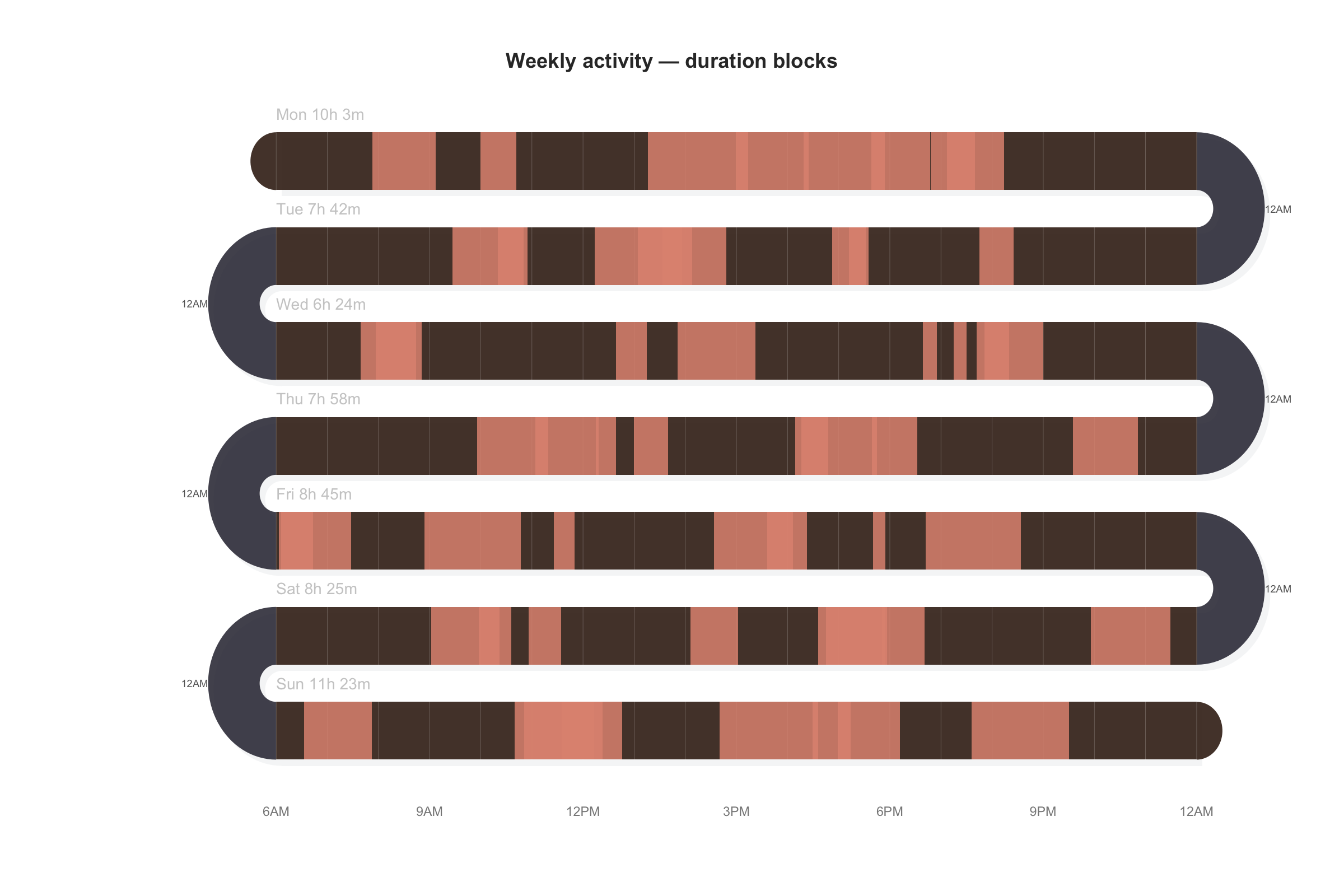
Activity timeline: Events across the week

Daily activity logs—app usage, study sessions, exercise bouts—are naturally continuous within a day but disconnected across days. Plotting seven days as separate 24-hour axes makes it hard to compare the same time slot across days; a single concatenated axis loses the day boundaries entirely. The serpentine layout gives each day a full-width 24-hour ribbon, with colored blocks showing event durations and rug ticks marking point events. Days flow into each other through the arcs, so weekly rhythms (weekday clusters vs. weekend gaps) become immediately visible.

activity_snake(events, event_color = "#e09480",
               band_color = "#3d2518",
               title = "Weekly activity — duration blocks")

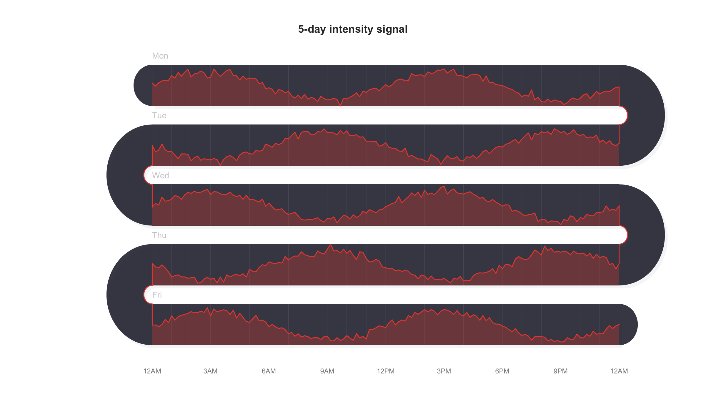
Continuous signal: Line intensity

Continuous signals recorded over multiple days—heart rate, screen time, sensor readings—pose a display dilemma: a single long axis compresses five days of minute-level data into an unreadable smear, while separate panels disconnect the end of one day from the start of the next. The serpentine layout threads the intensity curve through stacked bands connected by arcs, so the signal is literally continuous from band to band. Peaks and valleys are easy to trace across days, and the folded layout fits a week of high-resolution data into a single compact figure.

line_snake(d_line, fill_color = "#e74c3c",
           title = "5-day intensity signal")